To observe the trends within a dataset, we can perform a squared average or simple average. Instead, let say there is a situation where you need to prioritize a few data points over the rest. Like in predicting the temperature requires us to prioritize the latest values. Exponentially Weighted Moving Averages (EWMA) helps us in solving problems like this.

EWMA weighs the latest or recent data points with higher weights or magnitude than the rest of the data points as an exponential function. The graph below is a plot of temperatures in New Jersey throughout the year.

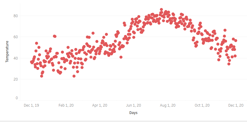
As mentioned earlier one way to identify the trend among these noisy data points would be simple averages. So what is the problem with that approach? Well, you can see that a simple average would consider all the data points with equal significance.

For instance, in this scenario consider the temperatures at Feb 2020 and August 2020. There is a lot of difference and the current day’s temperature depends more on say last 10 days than on the temperature three months ago.

How to calculate the moving averages?

This problem of all data points with the same weight is solved by E.W.M.A, where we have a hyperparameter β also called a smoothing parameter as it helps to reduce the noise in data.

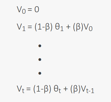
The θ values are the temperatures, the image shows the calculation of moving averages V where (β < 1). The magnitude of θ is 1- β and V is β. So, when β = 0.9, that means we are trying to average among 10 (1/(1-β)) recent V values.

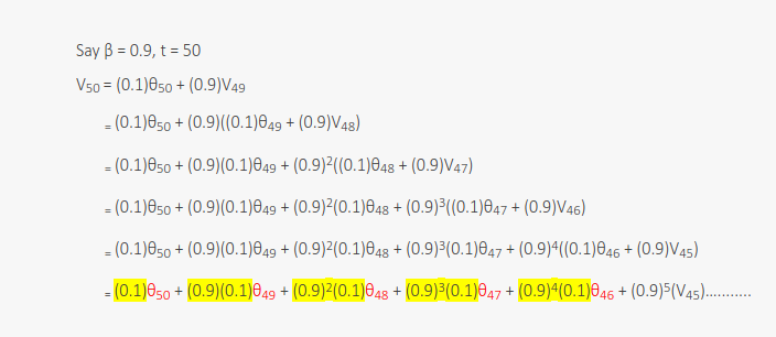
Now, when β = 0.9 and t = 50, the above calculations show how the magnitude of θ penalizes. From this calculation we can say two things:

• The magnitude of θ rises depending on how recent the data point is.

• The decrease of this magnitude is exponential.

The trends of temperature for different values of β are shown above, we can draw the following observations:

• For β = 0.98 we are averaging the 50 recent values, as a result, it is a smooth graph compared to the graph of β = 0.9.

• Also, we can see a shift in β = 0.98 graph this is due to averaging against the large group of values with high weights and less weights to the current temperature, adaption becomes tough.

• For β = 0.9 we are averaging the latest 10 values, and as seen the blue graph tends to have reduced the noise.

• For β = 0.5 we are averaging two recent values, due to which there is a lot of noise compared to both the previous values.

In the conclusion, the exponentially weighted averages would allow us to tune one more hyperparameter β. Through this, we can put more weights on the 1/1-β number of recent values than the rest of the values. One thing to observe in the above graphs is how they all started from 0 and took some time to take over the average values, this phenomenon is called Bias Variance which I will explain in my next post.